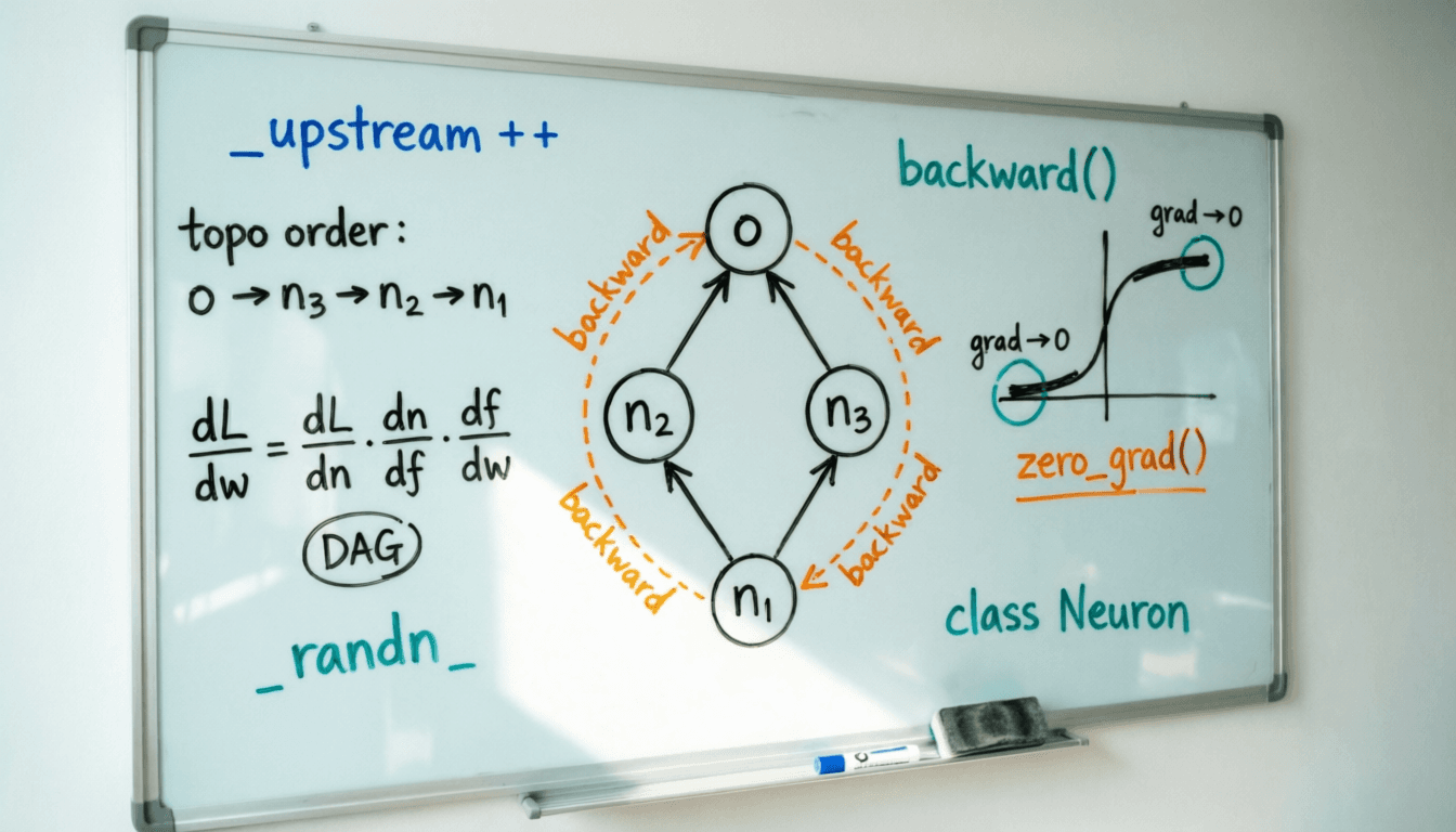
The biggest neural networks you have heard of are all trained using a deep learning framework like PyTorch or JAX. All of them have something like a .backward() function, either with a model or with the loss function, which then runs the most important part of model training: the backpropagation.
In PyTorch, you even have to add an optimiser.zero_grad() step right before you run the backward function. The framework itself handles the rest. Just removing these two lines would literally break your entire training loop. There is an entire story just in what happens behind the scenes of these two lines - something which we will explore today!
💡
This is part 2 of Building neural networks from scratch. If you haven't read the first part yet, I'd strongly suggest you read it now before you proceed with this blog because our understanding continues from the first part of the blog. For the notebooks, check out the GitHub here.
In this blog, we're going to write our own autograd engine from scratch on our Neuron class, and use it to train a classification model on the Iris dataset. We will explore what exactly an autograd engine is and why it is important to have one in our Neural network.
Before we get started with building an autograd engine, we have to fix a serious bug that exists in our current Neuron class.
The Vanishing of Gradients
I discovered this bug while training an MLP on the Iris dataset (more on this at the end of the blog). Turns out this is a very deep issue that can be solved by just changing how we initialise weights.
The problem
Previously, we initialised the weights and biases through this:
class Neuron:
	def __init__(self, inputs=[], act='relu') -> None:
	... initialising inputs
	self.weights = np.random.random(len(self.inputs))
	self.bias = np.random.random()
	... other initialisations
We're using the np.random.random() method. This returns a random number in interval. Our weights are only initialised with positive numbers.
[0.0,1.0)
Our choice of activation function plays a very important role here. I have shown the plots of sigmoid and tanh in my previous blog, which 'compress' all the input values to very specific ranges (0,1) and (−1,1) respectively.
If we get a very large or very small dot product which goes through these activation functions, the differentials of these activation functions would be close to 0.
In the case of training on the Iris dataset, the choice of activation function is tanh. And since the weight and the dot product are very large, our value of tanh gets close to 1.
And what is the differential of tanh?
dxdtanh(x)=1−tanh2(x)
Here is the plot of tanh once again, along with the plot of it's derivative.
Clearly, the differential of our neuron value will approach close to 0 as the value of tanh approaches either 1 or -1.
This means all of our gradients will be closer to zero. This is a very famous problem you would typically encounter while training any type of neural network. It is called the vanishing of gradients.
Why is this a problem?
If our gradients are approaching zero, so is our upstream. Applying these differential values in the chain rule, our entire expression becomes infinitesimally small.
E.g.
If dw1dL=dn1dL⋅df1dn1⋅dw1df1 and df1dn1→0then dw1dL→0
We have practically lost the information about how much the loss L is dependent upon the weight w1, only because one of the terms in the expression was close to 0.
This results in a very unstable training, the model struggles to update the weights properly and the end result is our model performing extremely poorly.
Had our weights been initialised all negative, we would see the same results: the values of tanh would be approaching -1 and the differential would still be close to 0.
Using larger weights
When I encountered this bug, I honestly wondered: "If the gradients are approaching zero, then why not initialise very large weights? That way, the differentials with very small value is compensated with larger weights. So Simple!"
Very clever, but here's the thing: initialising parameters with extremely large values would result in a totally new problem called exploding gradients.
Unlike vanishing gradients where the gradients get close to 0, we get gradients which have extremely large values. And this is another problem when updating the weights.
wnew=wold−η∂w∂L
If the loss gradient is extremely large, the new weights would update by a large value which can very easily overshoot the minima.
Furthermore, even the most powerful computers in the world can store finite range of data. If our values cross that limit, then either the computer would crash or we would get a NaN (Not a Number). And once you get that, there's no going back!
So turns out initialising our weights to be very large doesn't help either!
So how exactly do we fix this?
The real fix
There are many ways with which we can fix this. But for the scope of our blog, we have the easiest and most obvious fix.
All we have to do is update our weight and bias initialisation:
# Before
self.weights = np.random.random(len(self.inputs))
self.bias = np.random.random()

# After
self.weights = np.random.randn(len(self.inputs))
self.bias = np.random.randn()
The difference between random() and randn() is that former generates floats from the Uniform Distribution from 0 to 1, while the latter draws numbers from the Gaussian Distribution with the mean of 0 - where 68% of the time the values generated are in between [−1,1].
In simple words, a NumPy array using random() would have an average greater than 0 since all the numbers are positive, whereas the array generated by randn() has positive and negative numbers. Mixed signs help us control the weights so that dot product is close to 0.
Because of the nature of tanh activation function, we want our values to be around 0 which is exactly where randn() helps us. The correct initialisation of weight with the activation function in mind is super important.
💡
This simple solution works only for our use case. In production systems when you are working with large scale networks, you would use techniques like Batch Normalisation and Residual Connections. You also might want to look at different types ofweight initialisations that depend on the activation function.
Now with that fixed, let's start building our autograd engine!
Building an Autograd engine
Now for the main part of the blog: writing an autograd engine. An autograd engine is an algorithm that automatically computes and stores the gradients of every neuron in a network, without us having to manually rewrite the backpropagation algorithm.
Let's work with a very small neural network, implement the topological sort and write our engine:
This is a very simple network which takes a single number through n1, then it links to n2 and n3 and finally both merge to output neuron o.
A quick recap
A neural network learns data and its patterns through an algorithm called 'backpropagation'. Backpropagation is an algorithm which updates the parameters of a neural network by calculating gradients.
These gradients are basically the rates of change of the loss value with respect to the weights and biases for each neuron, and their mathematical expressions are evaluated with the help of the Chain rule.
To check how much the model's predictions are different from the actual outputs, we calculate the model loss. As an example for any neuron nx with a weight wx, if we wanted to find out how much the model loss L is changing w.r.t wx :
∂wx∂L=∂nx∂L⋅∂fx∂nx⋅∂wx∂fx
One of the goals in model training is to minimise this loss value so that our model's predictions match the real outputs as much as possible.
The motivation
In our Part 1, we defined a Neuron class that does exactly this: computes the loss, finds out the gradients and updates the weights. However, we had to manually implement the backward pass and pass the new upstreams one by one.
If we write our backward pass for our diamond network for single iteration:
Note: We are accumulating the upstream of n1 by adding dL_dn1_dn2 and dL_dn1_dn3 since both n2 and n3 are going back to n1 to satisfy the chain rule.
Remember the gradients of n1 that we are getting after a single iteration: [-0, -181.5179154]. We will use this to verify whether our autograd engine is working later or not.
We can notice that each neuron is dependent on its succeeding neuron. We cannot calculate a neuron's gradients unless we have its succeeding neuron's gradients calculated and upstream ready. We also have to ensure that the order in which we update the gradients is correct, and this makes manual backprop even harder.
For small networks, this is tedious but still doable. But as the networks grow larger and larger, it would become more difficult to keep track of the calculations.
What if there were an algorithm that ensures that the upstream is passed to the chain of neurons in the correct order, and the gradients are calculated and updated while we are traversing through a neuron?
Neural Networks as Graphs
If you think about it, neural networks are basically large-scale graph data structures. More specifically, they are Directed Acyclic Graphs where each node (neuron) is pointing towards another node in such a way that there are no cycles or closed loops in the entire graph.
The neurons are nodes and the connections are edges. This means that all the graph-related algorithms, such as Depth First Search, are applicable here.
The algorithm that can help us here is Topological Sort. More specifically, we are going to use Reverse Topological Sort in a DFS manner. This algorithm is what really powers our autograd engine.
Topological sort
A topological sort is a Graph Algorithm which ensures that all the nodes in the graph are arranged in a linear sequence in such a way that the nodes are traversed in a specific order. In backpropagation, since we are going from the output neuron to the leaf neurons, we are going in the reverse direction from end to start.
We can write the code for topological sort in Python for our Neuron:
def topo_sort(output):
	# it can either be a neuron or a layer
	order = []
	visited = set()

	def build_order(output: Neuron):
		if output not in visited:
			visited.add(output)
			for inputs in output.input_sources:
				# check if the input is a number or another neuron
				if callable(inputs):
					build_order(inputs)
			order.append(output)

	if callable(output):
		# it's a neuron
		build_order(output)
	else:
		# it's a layer
		for k in output:
			build_order(k)

	return order[::-1]
The output can either be a single neuron or it can be an array of neurons as a single layer. This code handles both of the cases, builds an order to traverse the neurons and returns the reversed order.
If we run the topological sort in our small network, we get an array which tells us the order in which we have to traverse.
Note: For this particular graph, the order can also be [o, n2, n3, n1] since there are two ways to get to the neuron n1. Both of the ways are equally correct and will not affect our calculations.
Updating our backward pass
Let's first rename our .backward() method as ._compute_grad_upstream(), as we're going to add a new .backward() method. This makes it clear that our function currently is computing gradients and the new upstream.
We also add another class variable called self._upstream in our Neuron class. This variable stores the neuron gradient: ∂n∂L of a particular neuron n. This neuron gradient can act as the upstream for its preceding neurons for their gradient calculation.
class Neuron:
	def __init__(self, name, inputs=[], act='relu') -> None:
		...
		self._upstream = 0    # new class variable
		...

	... other methods

	def _compute_grad_upstream(self,upstream):
		... renaming our backward method, the code stays the same
		# another thing to return, the new upstream: loss gradient with respect to previous neurons' output
		new_upstream = upstream * d_act * self.weights
		return new_upstream

	def backward(self, seed):
		... new backward pass

	@staticmethod
	def layer_backward(layer, seed):
		... new backward pass for handling layer
We will fill in these new methods in a little bit. I'm handling both cases at the same time: whether the output is a single neuron or we have an output layer. The underlying logic is going to be the same in both cases.
For now, if you remember, we are computing the new upstream variable for the current neuron and returning it from the function so that we can pass it to preceding neurons. The mathematical formula for this is as follows:
∂nprev∂L=∂nx∂L⋅∂fx∂nx⋅∂x∂fx
where:
∂nprev∂L is the new upstream returned as new_upstream
∂nx∂L is the upstream accessed as upstream variable
∂fx∂nx is the differentiation of the activation function computed in and finally,
∂x∂fx is the differential of the dot product with respect to inputs, which simply is the weight.
So far, we returned the new upstream from the function and we had to use that value as the seed to its preceding neuron's backward method (which is now ._compute_grad_upstream.)
Now, new_upstream is a NumPy array because the current Neuron stores the upstream variables for multiple preceding neurons i.e. our current neuron can have multiple inputs, so we store the upstream for each of those inputs.
We don't have to return this NumPy array, we can directly update the _upstream for each of those input neurons directly via the input_sources class variable.
# return new_upstream.  -> we don't need this anymore

# update the upstream for each preceding neurons
for i, inps in enumerate(self.input_sources):
	if callable(inps):    # check if the input is a neuron
		inps._upstream += new_upstream[i]
Notice again that we are accumulating the upstreams to ins._upstream again. If you calculate the upstream using the chain rule, you would end up with the same result. As mentioned before, a neuron can feed its output to multiple neurons, and each of those neurons is going to give back its own upstream, which we have to simply add.
Finally, our class method only takes an upstream variable as an input, computes the loss gradients and sets its input neurons' loss gradients directly.
The new .backward methods
We explored what topological sort is earlier. We can use it to determine which neurons have to be updated first in order. We can start our backward pass by simply iterating through this order and computing each of those neurons' gradients.
def backward(self, seed):
	order = topo_sort(self)

	self._upstream = seed   # set the seed as current neurons upstream

	for node in order:
		node._compute_grad_upstream(node._upstream)
But what if our Neural network has multiple output neurons in a layer? Again, we can define a Python staticmethod to write out the backward pass: set the upstream for each output, find out the correct order, compute the gradients and set the input upstreams.
@staticmethod
def layer_backward(layer, seed):
	# seed the output layers first
	for o_i, s_i in zip(layer, seed):
		o_i._upstream = s_i

	# find out the order
	order = topo_sort(layer)

	# walk through the order
	for node in order:
		node._compute_grad_upstream(node._upstream)
Verification of the new backward pass
Let's use these new .backward methods that we just defined in our diamond neural network. Instead of calculating the new upstreams for different neurons and passing them to each _compute_grad_upstream method, all we have to do is seed the .backward only once.
If you notice, the value of n1.gradients is the same as what we obtained before manually. This means the gradients are calculated in the right order, and our logic is working correctly. Our autograd engine is ready!
💡
Though this engine only works for our own customNeuron class, the underlying concepts and the core logic remain the same. It is not fully 'battle-tested', and it may or may not work in certain edge cases. The whole point is to understand how backpropagation works when training large neural networks, and what happens behind PyTorch's loss.backward().
In production frameworks such as PyTorch, you would want to move this process from being executed on the CPU to more specialised hardware such as a GPU or a TPU. In that case, you write this in a low-level language like C++ or CUDA and make the function calls from Python.
That is an advanced-level project which we are not going to cover here. If you happen to have a GPU, you can try to implement our network by writing kernels, which can significantly speed up the model training!
Zeroing out the gradients
At the end of part 1, I presented a challenge: to train an MLP using the Neuron class on the
Iris dataset. Let's attempt the challenge and see if our engine is working correctly!
Using our new and updated Neuron class with the new backward() method, here's the model architecture that I came up with:
Seems a bit messy, but it's just every neuron of one layer connected to every neuron in the succeeding layer. The Python code for the above architecture:
np.random.seed(0)
layer1 = [Neuron(name=f'l1_{i}',inputs=[0,0,0,0], act='tanh') for i in range(8)]
layer2 = [Neuron(name=f'l2_{i}',inputs=layer1, act='tanh') for i in range(6)]
output = [Neuron(name=f'o_{i}',inputs=layer2, act='linear') for i in range(3)]
To calculate the model loss, we're going to use Cross Entropy Loss as it best measures the distance between the two output probabilities: real and predicted. The output probabilities are obtained via the Softmax function, which takes the model's raw output scores from 3 neurons and returns a probability distribution.
def softmax(logits):
	exp = np.exp(logits - np.max(logits))
	return exp / np.sum(exp)

def cross_entropy_loss(pred, real):
	upstream = pred - real
	eps = 1e-10 # small epsilon delta to avoid log(0) errors
	loss = -np.sum(real * np.log(pred + eps))
	return loss, upstream
Inside the training loop, we're going to use Neuron.layer_backward, since the final output is a layer rather than a single neuron.
I have set the hyperparameters learning rate as 1e-3 and the number of iterations as 400. On running the training loop and plotting the loss and accuracy, we get the following plots:
These plots look very interesting! Our model is updating the gradients correctly, and the training loop is running without any issues. Initially, the training seems to be quite unstable. But as it slowly becomes more stable, our model seems to struggle to learn the data.
The accuracy goes up very slowly, and the loss reaches a baseline value of almost 1.0987. If we simply print out the accuracy in another cell, we get 0.34. Which means our model is predicting the correct values 34% of the time.
We can see this by running the testing code as below:
# pick a random index from the dataset
idx = np.random.randint(0, 150)
x_test = x[idx]
y_test = y[idx]

print("Random index choosen:", idx)

for l in layer1:
	l.set_input(x_test)
logits = np.array([o() for o in output])
probs = softmax(logits)
category = np.argmax(probs)

predicted = iris_dataset.target_names[category]
actual = iris_dataset.target_names[np.argmax(y_test)]

print(f"Predicted: {predicted}, Actual: {actual}")
So our engine is working correctly, the weights are being updated correctly, but the model is still unable to learn properly.
Why is our model unable to learn?
So far, we have only optimised the backward pass so that it performs automatically. We have not made any changes to the model training.
The real culprit is that we are not zeroing out our gradients at all. After every iteration, all those upstreams simply add to the existing upstreams from previous iterations, which is why our parameters are not being updated properly.
This wasn't an issue in Part 1. We were writing the backward pass ourselves by manually overwriting self.gradients, and the upstream was being passed to the next neurons manually.
Building the autograd engine forced us to introduce an _upstream class variable, and the only way a neuron can collect gradients from multiple downstream paths is by adding them. This accumulation is what makes the engine work correctly.
As we can see, this zeroing out and resetting of the gradients and the upstream becomes necessary.
We now add one final method to our Neuron class:
def zero_grad(self):
	# reset the gradients to zero to avoid gradient accumulation
	self.gradients = np.zeros(len(self.weights) + 1)
	self._upstream = 0
We are resetting the upstream to be zero as well, which is optional since they are overwritten according to our design choice anyway, and so only resetting the gradient variable is essential here. But real frameworks accumulate gradients and upstreams too (when dealing in batches of data), so zeroing out both of them is a good practice.
Call this class method right before the backward pass. I'm zeroing out the gradients for each neuron manually, but you could further optimise it and zero out the gradients by the topological order too:
# get model loss
L, dl_do = cross_entropy_loss(out_probs, y_train)

# zero out the gradients
for o in output:
	o.zero_grad()
for l2 in layer2:
	l2.zero_grad()
for l1 in layer1:
	l1.zero_grad()

Neuron.layer_backward(output, dl_do)
Now, if we retrain our model, we get a much better plot, and our model is finally able to learn:
We get the model accuracy of ~98% - the predictions are much better than before!
💡
Do not get confused about zeroing out the gradients by resetting the 'learning progress' of the model. A model's knowledge lives in the parameters. Gradients just indicatein which direction the parameters should be updated. Once the step function updates the weights, the gradients are no longer needed.
So finally, we have completed all the necessary steps required for model training on the Iris dataset. Our autograd engine is working correctly, the gradients are updating properly, the model is learning, and the predictions are coming out right.
Conclusion
In Part 1 of this blog, we learned what a Neuron is exactly and how we can have multiple neurons linked with each other to form a deep neural network.
We took that same Neuron class where we had to write the backward pass manually by hand for each neuron, into one single .backward() call that differentiates the entire network.
To sum up:
We fixed a bug in our Neuron class by reinitialising the weights in a normal distribution around zero, which keeps the gradients alive and avoids saturating the tanh activation function. By keeping the dot products in tanh's optimal range, we have fixed the vanishing gradients problem.
We also learnt not to initialise the weights with extremely large values, as this can result in an explosion of gradients, which drastically updates the weights and easily overshoots the loss minima.
Neural networks are Directed Acyclic Graphs. Backpropagation is now a graph traversal algorithm where the reverse topological sort ensures a neuron's gradients are only computed once every neuron it feeds to has computed theirs. It is the topological sort + chain rule which truly powers our autograd engine.
After the forward pass and before the backward pass, it is important to zero out the gradients and upstream to ensure the gradients don't accumulate from previous iterations, with which the model can struggle to learn the data. It is an important step in model training.
We have 5 basic steps in model training:
Forward pass: The data passes through the model, and the model predicts an output.
Loss calculation: We calculate how far the predictions are from the real values to evaluate the model's performance.
Zeroing gradients: Clearing the previous iteration's gradients and the upstream before the backward pass sets them according to the loss.
Backward pass: Find out how much the loss would change with respect to each weight, bias, and neuron's output and store them as gradients.
Update parameters: Using those gradients, we update the model parameters with a small learning rate.
Neural networks are not magic - it's all just math, and we did it ourselves. It simply runs on a CPU, one sample at a time. Our engine is nowhere near PyTorch, but the core principles remain the same.
I hope these two blogs helped you gain a solid understanding of what neural networks really are. We have finally built, trained and optimised our Neural network - from first principles!🚀✨